The following article will give you step by step instructions on how to build and demo a Power View report using CRM data. Note that you can do this with CRM Online and On Premise. You do not have to have SQL 2012 or SharePoint installed!
A great deal of thanks for this article goes to my colleague Huw Edmunds from Microsoft Consulting Services (MCS). Huw has devoted many hours of his own time helping me with SQL 2012 and Power View. In a future post I hope to convince Huw to help me write a simple set-up guide for SQL 2012, SharePoint and Power View for On Premise demo’s.
In this article I am going to provide you with the following files:
- The raw data to import into CRM PowerViewOppsImportFile
- An Example Power View report created from the same raw data PowerViewOppsExample
I have two demonstrations on my laptop that I use to show Power View:
- CRM 2011 On Premise VPC running SQL 2012, SharePoint 2010 and Excel 2010 (thanks Huw!)
- CRM Online running Microsoft Excel 2013
I am not going to cover the set-up of SQL 2012 and Power View (that is for another post) but I will provide you with the data and steps to create a meaningful demo. If you do not have an On Premise instance with SQL 2012 then you will need to install Excel 2013. Note that you can run Excel 2013 alongside Microsoft Excel 2010 (you cannot run two versions of Outlook however).
So for the purpose of the remainder of this article I am going to assume:
- You already have an organisation on CRM Online
- You have installed Microsoft Excel 2013
Step by step instructions for creating a Power View Demo with CRM Online and Excel 2013:
- Download the Opportunity data (open the file and save as CSV) here: PowerViewOppsImportFile
- Create and publish a new field on the Opportunity Entity called “Days To Close”
- Import the data into your CRM online instance
- Using Advanced Find create a view in CRM with the data you have just imported (I used all Opps created on XYZ date)
- From the view you have just created, export the data to an Excel file. Make sure that you save the file (or rename after export) to xlsx
- Open the Excel file you have just exported. You should have something like this PowerViewOppsExample, and select all the columns (A to F)
- Note: I had to rename the field I wanted to use for the location to start with the word “City”, if you do not do this Power View may not display the location properly.
- From the ribbon select Insert Table
- From the ribbon select insert Power View
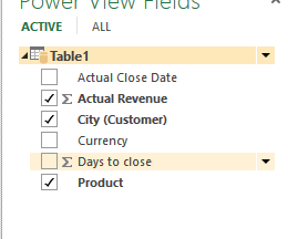
- Uncheck/Check only the following fields (Actual revenue, City, Product)
- Select Column Chart
- Select Map (in a demo I like to show this view as the column chart first and then show how it turns into a map

For the scatter chart:
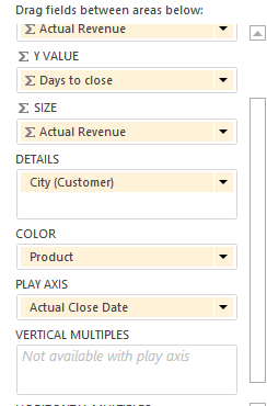
- Drag the following fields (actual Revenue, Days to Close, City, Product, Actual Close date ) below the existing chart (this will create a new table)
- Select the table and turn it into a scatter chart (under Other Chart on the Ribbon) and set the chart as follows
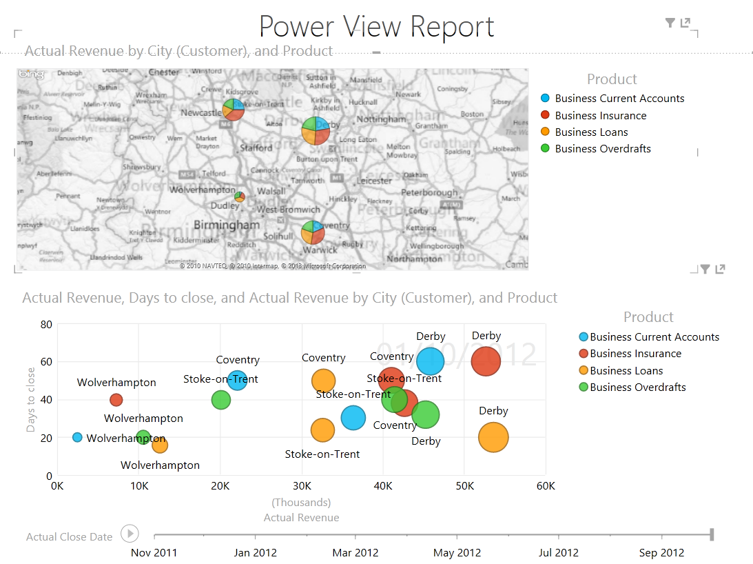
 So you should end up that looks like this:
This posting is provided “AS IS” with no warranties, and confers no rights.
Next week on Mark Margolis’s Blog: XRM for Financial Services
